막연한 꿈 금융시계열 마스터해서 부자되기
의 첫스텝의 첫스텝 LSTM time series forecasting이다
사실 저번주 쯤에 한 번 시도해 봤는데, 텐서가 뭔지, 차원이 뭔지도 잘 모르는 상태여서 안 했다고 봐도 무방할 정도다.. 그래서 아주 약간의 pytorch지식을 장착한 후 재도전한다.
lecture Reference : https://www.youtube.com/watchv=q_HS4s1L8UI&list=PLKYEe2WisBTHmsTdhjaQydI58tI7pFCDT&index=3
가르쳐주셔 감사함니다..
강의 따라한 Colab
https://colab.research.google.com/drive/1YXWyVCD6LxNXdWIvqI6iODfcpiH6Mcmt?usp=sharing
Google Colaboratory Notebook
Run, share, and edit Python notebooks
colab.research.google.com
import pandas as pd
import numpy as np
import matplotlib.pyplot as plt

import torch
import torch.nn as nn

data = pd.read_csv('AMZN.csv')

data
필요한 라이브러리들 import, 데이터 로드

데이터는 대충 이렇게 생겼다
가격이 극심하게 차이나는 이유는, 주식병합이나 액면분할 때문인 것 같다. 나중에 MinMaxScaler로 -1, 1사이로 전부 정규화 한다
# stock forecasting에 필요한 columns만 가져옴
data = data[['Date', 'Close']]
data

# training을 수행해야 하기에 GPU인 CUDA를 활용할 수 있는지 체크
device = "cuda:0" if torch.cuda.is_available() else 'cpu'
device

# string type의 'Date'를 pandas의 datetime객체로 변경
data['Date'] = pd.to_datetime(data['Date'])
data.head()

# 종가 그림
plt.plot(data['Date'], data['Close'])
from copy import deepcopy as dc

def prepare_dataframe_for_lstm(df, n_steps):
  df = dc(df)

  #set_index공부
  df.set_index('Date', inplace=True)

  for i in range(1, n_steps+1):
    df[f'Close(t-{i})'] = df['Close'].shift(i)

  #dropna : 결측치가 있는 부분 제거
  df.dropna(inplace=True)

  return df

# 며칠간의 widnow로 주가 예측할 것인가
lookback = 7
shifted_df = prepare_dataframe_for_lstm(data, lookback)
shifted_df

#inplace=False (기본 설정)으로 설정된 경우, 변경된 새 데이터프레임을 반환하고 원본 데이터프레임은 그대로 유지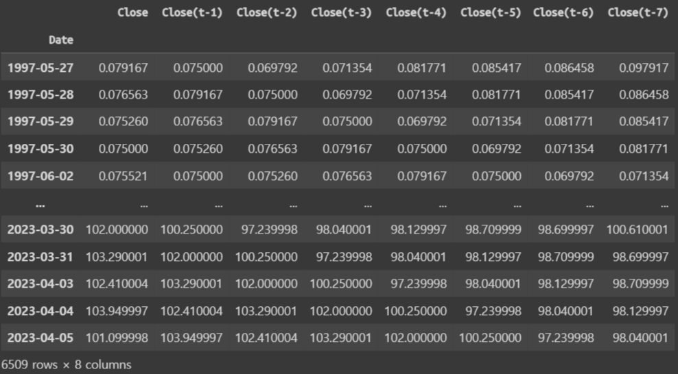
#scaling을 위해 dataframe 을 numpy로 바꾸어 줌
shifted_df_as_np = shifted_df.to_numpy()
shifted_df_as_np

shifted_df_as_np.shape
#>>>(6509, 8)

from sklearn.preprocessing import MinMaxScaler

#(-1, 1) MinMaxScaling
scaler = MinMaxScaler(feature_range = (-1, 1))
shifted_df_as_np = scaler.fit_transform(shifted_df_as_np)
shifted_df_as_np

X = shifted_df_as_np[:, 1:]
y = shifted_df_as_np[:, 0]

X.shape, y.shape
#>>>((6509, 7), (6509,))
#LSTM의 input으로 최근 내용이 나중에 들어가야 예측이 더 수월함
# t-1 -> t-2 ... -> t-7에서
# t-7 -> t-6 ... -> t-1로 바뀌면서 최근 주가가 나중에 들어감
X = dc(np.flip(X, axis = 1))
X
"""
array([[-0.99969839, -0.99982128, -0.99983244, ..., -0.99998325,
-1. , -0.99995531],
[-0.99982128, -0.99983244, -0.99987154, ..., -1. ,
-0.99994415, -0.99991063],
[-0.99983244, -0.99987154, -0.99998325, ..., -0.99994415,
-0.99989946, -0.99993855],
...,
[ 0.05779984, 0.05158 , 0.0506149 , ..., 0.07431453,
0.09308121, 0.10690997],
[ 0.05158 , 0.0506149 , 0.04203581, ..., 0.09308121,
0.10691495, 0.09747299],
[ 0.0506149 , 0.04203581, 0.07431453, ..., 0.10691495,
0.09747802, 0.11398769]])
"""# train, test set 분리
split_index = int(len(X)*0.95)
split_index
# 6183
X_train = X[:split_index]
X_test = X[split_index:]
y_train = y[:split_index]
y_test = y[split_index:]
X_train.shape, X_test.shape, y_train.shape, y_test.shape
# ((6183, 7), (326, 7), (6183,), (326,))#(데이터수, 참조할주가수, 예측치1개)
X_train = X_train.reshape((-1, lookback, 1))
X_test = X_test.reshape((-1, lookback, 1))
y_train = y_train.reshape((-1, 1))
y_test = y_test.reshape((-1,1))
X_train.shape, X_test.shape, y_train.shape, y_test.shape
# ((6183, 7, 1), (326, 7, 1), (6183, 1), (326, 1))
X_train = torch.tensor(X_train).float()
X_test = torch.tensor(X_test).float()
y_train = torch.tensor(y_train).float()
y_test = torch.tensor(y_test).float()
X_train.shape, X_test.shape, y_train.shape, y_test.shape
"""
X_train = torch.tensor(X_train).float()
X_test = torch.tensor(X_test).float()
y_train = torch.tensor(y_train).float()
y_test = torch.tensor(y_test).float()
X_train.shape, X_test.shape, y_train.shape, y_test.shape
(torch.Size([6183, 7, 1]),
torch.Size([326, 7, 1]),
torch.Size([6183, 1]),
torch.Size([326, 1]))
"""from torch.utils.data import Dataset
class TimeSeriesDataset(Dataset):
def __init__(self, X, y):
self.X = X
self.y = y
def __len__(self):
return len(self.X)
def __getitem__(self, i):
return self.X[i], self.y[i]
train_dataset = TimeSeriesDataset(X_train, y_train)
test_dataset = TimeSeriesDataset(X_test, y_test)
train_dataset
# <__main__.TimeSeriesDataset at 0x7eb9ef630be0>
from torch.utils.data import DataLoader
batch_size = 16
train_loader = DataLoader(train_dataset, batch_size=batch_size, shuffle=True)
test_loader = DataLoader(test_dataset, batch_size=batch_size, shuffle=False)
#batch_index는 안 필요해서 underline
for _, batch in enumerate(train_loader):
x_batch, y_batch = batch[0].to(device), batch[1].to(device)
print(x_batch.shape, y_batch.shape)
# 첫 번째 batch만 확인
break
# torch.Size([16, 7, 1]) torch.Size([16, 1])# LSTM class define
class LSTM(nn.Module):
def __init__(self, input_size, hidden_size, num_stacked_layers):
super().__init__()
#hidden_size, num_stacked_layers는 forward함수에서 다시 사용되기 때문에 인스턴스 초기화
self.hidden_size = hidden_size
self.num_stacked_layers = num_stacked_layers
self.lstm = nn.LSTM(input_size, hidden_size, num_stacked_layers,
batch_first = True)
self.fc = nn.Linear(hidden_size, 1)
#텐서 차원을 이렇게 선언한 이유는 잘 모르겠음..
def forward(self, x):
batch_size = x.size(0)
h0 = torch.zeros(self.num_stacked_layers, batch_size, self.hidden_size).to(device)
c0 = torch.zeros(self.num_stacked_layers, batch_size, self.hidden_size).to(device)
out, _ = self.lstm(x, (h0, c0))
out = self.fc(out[:, -1, :])
return out
model = LSTM(1,4,1)
model.to(device)
model
"""
LSTM(
(lstm): LSTM(1, 4, batch_first=True)
(fc): Linear(in_features=4, out_features=1, bias=True)
)
"""# Train one Epoch
def train_one_epoch():
model.train(True)
print(f'Epoch: {epoch + 1}')
running_loss = 0.0
for batch_index, batch in enumerate(train_loader):
x_batch, y_batch = batch[0].to(device), batch[1].to(device)
output = model(x_batch)
loss = loss_function(output, y_batch)
running_loss += loss.item()
optimizer.zero_grad()
loss.backward()
optimizer.step()
if batch_index % 100 == 99: # print every 100 batches
avg_loss_across_batches = running_loss / 100
print('Batch {0}, Loss: {1:.3f}'.format(batch_index+1,
avg_loss_across_batches))
running_loss = 0.0
print()def validate_one_epoch():
model.train(False)
running_loss = 0.0
for batch_index, batch in enumerate(test_loader):
x_batch, y_batch = batch[0].to(device), batch[1].to(device)
with torch.no_grad():
output = model(x_batch)
loss = loss_function(output, y_batch)
running_loss += loss.item()
avg_loss_across_batches = running_loss / len(test_loader)
print('Val Loss: {0:.3f}'.format(avg_loss_across_batches))
print('***************************************************')
print()#model train
learning_rate = 0.001
num_epochs = 10
loss_function = nn.MSELoss()
optimizer = torch.optim.Adam(model.parameters(), lr=learning_rate)
for epoch in range(num_epochs):
train_one_epoch()
validate_one_epoch()
"""
Epoch: 1
Batch 100, Loss: 1.250
Batch 200, Loss: 0.170
Batch 300, Loss: 0.028
Val Loss: 0.018
***************************************************
Epoch: 2
Batch 100, Loss: 0.005
Batch 200, Loss: 0.005
Batch 300, Loss: 0.004
Val Loss: 0.013
***************************************************
Epoch: 3
Batch 100, Loss: 0.004
Batch 200, Loss: 0.004
Batch 300, Loss: 0.003
Val Loss: 0.011
***************************************************
Epoch: 4
Batch 100, Loss: 0.002
Batch 200, Loss: 0.003
Batch 300, Loss: 0.002
Val Loss: 0.011
***************************************************
Epoch: 5
Batch 100, Loss: 0.002
Batch 200, Loss: 0.002
Batch 300, Loss: 0.002
Val Loss: 0.010
***************************************************
Epoch: 6
Batch 100, Loss: 0.001
Batch 200, Loss: 0.001
Batch 300, Loss: 0.001
Val Loss: 0.009
***************************************************
Epoch: 7
Batch 100, Loss: 0.001
Batch 200, Loss: 0.001
Batch 300, Loss: 0.001
Val Loss: 0.007
***************************************************
Epoch: 8
Batch 100, Loss: 0.000
Batch 200, Loss: 0.000
Batch 300, Loss: 0.000
Val Loss: 0.006
***************************************************
Epoch: 9
Batch 100, Loss: 0.000
Batch 200, Loss: 0.000
Batch 300, Loss: 0.000
Val Loss: 0.005
***************************************************
Epoch: 10
Batch 100, Loss: 0.000
Batch 200, Loss: 0.000
Batch 300, Loss: 0.000
Val Loss: 0.005
***************************************************
"""with torch.no_grad():
predicted = model(X_train.to(device)).to('cpu').numpy()
plt.plot(y_train, label='Actual Close')
plt.plot(predicted, label='Predicted Close')
plt.xlabel('Day')
plt.ylabel('Close')
plt.legend()
plt.show()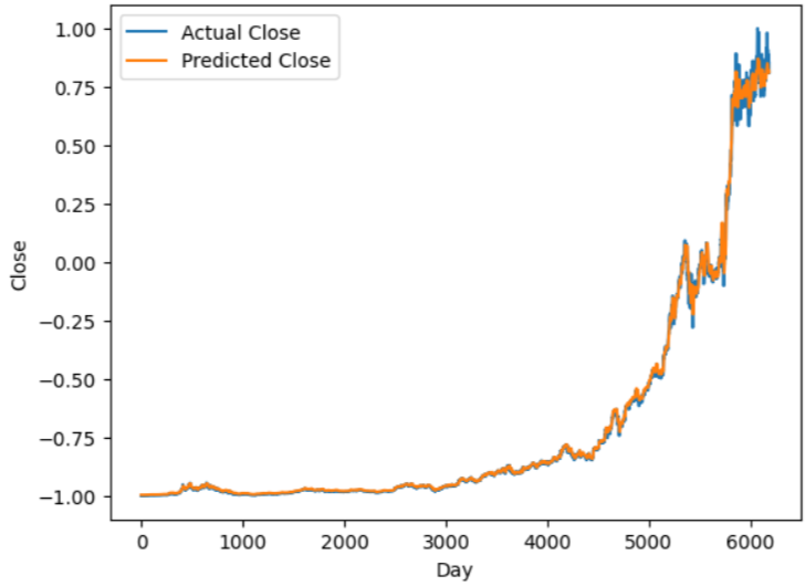
예측값 - 주황색
잘 예측하는 것 같음 but! scaling되어있는 상태라 실제 가격을 모름. 이제 스케일러 풀어주자
train_predictions = predicted.flatten()

dummies = np.zeros((X_train.shape[0], lookback+1))
dummies[:, 0] = train_predictions
dummies = scaler.inverse_transform(dummies)

train_predictions = dc(dummies[:, 0])
train_predictions
"""array([  0.47217395,   0.4699507 ,   0.46879461, ..., 169.15940866,
       168.86965258, 169.08869821])"""

dummies = np.zeros((X_train.shape[0], lookback+1))
dummies[:, 0] = y_train.flatten()
dummies = scaler.inverse_transform(dummies)

new_y_train = dc(dummies[:, 0])
new_y_train
"""array([7.91646265e-02, 7.65634249e-02, 7.52572660e-02, ...,
       1.69091505e+02, 1.73315001e+02, 1.68871003e+02])"""

plt.plot(new_y_train, label='Actual Close')
plt.plot(train_predictions, label='Predicted Close')
plt.xlabel('Day')
plt.ylabel('Close')
plt.legend()
plt.show()
test_predictions = model(X_test.to(device)).detach().cpu().numpy().flatten()

dummies = np.zeros((X_test.shape[0], lookback+1))
dummies[:, 0] = test_predictions
dummies = scaler.inverse_transform(dummies)

test_predictions = dc(dummies[:, 0])
test_predictions


dummies = np.zeros((X_test.shape[0], lookback+1))
dummies[:, 0] = y_test.flatten()
dummies = scaler.inverse_transform(dummies)

new_y_test = dc(dummies[:, 0])
new_y_test


plt.plot(new_y_test, label='Actual Close')
plt.plot(test_predictions, label='Predicted Close')
plt.xlabel('Day')
plt.ylabel('Close')
plt.legend()
plt.show()
파이토치 간략한 강의 듣고 다시 따라해 봤는데 확실히 이전보단 따라갈 수 있는 느낌이 강하게 들었음. 그런데 차원 설정이라던지, 스케일링 원상복구 하는 부분, 일부 메소드는 아직 정확히 이해하진 못한 것 같다. 코드 다시 복습하면서 메꾸어 나갈 예정이다.
또 하나, 아직 스스로 모델 설계를 해 보지 못했다. 모범답안 코랩 띄어 놓고, 흘끔 보고 나머지 코드 완성하고, 다음 순서 살짝 보고 코드 짜 보고 한 수준이다. 모델 훈련 및 validation의 큰 틀은 다르지 않을 것이니, 이 코드로 계속 공부하고 다른 factor들 추가해 보며 stock forecasting쪽 공부해 보겠다.


